The Inference Law

AI × Ham Radio

Ham radio is not really about radios. It is about antennas. And to understand antennas, you have to understand electricity — how voltage, resistance, and current relate to each other, and why changing one changes the others. That relationship is not obvious. Electricity is invisible. You cannot watch it move through a wire the way you can watch water move through a pipe.

This diagram is the one that helped it click for me while studying for my licence:

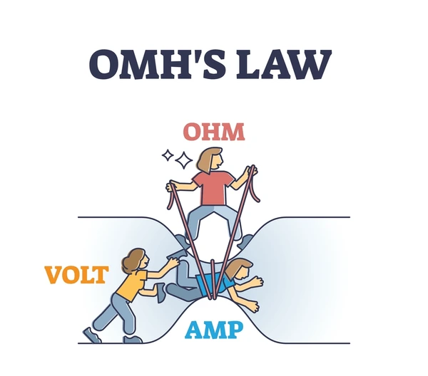
It is a little absurd. It is also immediately memorable. Voltage pushes, resistance holds back, current is what gets through. V = IR. Once you have seen it this way, the formula stops being arbitrary symbols and becomes a physical thing you can reason about. Increase the pressure, more gets through. Narrow the pipe, less gets through. The relationship is the same regardless of which variable you are solving for.

While writing last week's post on local AI hardware, I kept coming back to this diagram. The argument in that post is that memory bandwidth — not clock speed, not core count, not TOPS — is the metric that governs local AI inference. I was trying to explain why, and I realised I was describing the same kind of relationship: three variables, one formula, one diagram that makes it concrete.

I made this one:

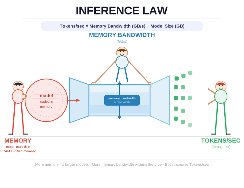
The formula is: Tokens/sec = Memory Bandwidth (GB/s) ÷ Model Size (GB).

The three variables work exactly like Ohm's Law. VRAM or unified memory capacity is the prerequisite — the model must fit entirely in VRAM or unified memory before inference can begin. If it does not fit, the model either cannot run at all, or spills into system RAM or NVMe storage, where memory bandwidth collapses and throughput falls with it. Memory bandwidth is the pipe: the rate at which the processor can pull model weights from VRAM or unified memory to calculate each token. And tokens per second is what you actually experience — whether a response feels instant or whether you are watching it type itself out one word at a time.

The formula is checkable. Apple's M4 Max has 410 GB/s of memory bandwidth. Running Llama 3.1 8B at Q4_K_M quantization puts approximately 4.7 GB into unified memory. Divide them: 410 ÷ 4.7 = 87 tokens/sec predicted. Measured real-world results on M4 Max for that model run between 64 and 92 tokens/sec. The formula works — and works well enough to plan hardware purchases around.

That is what I find striking about this formula compared to Ohm's Law: it is more concrete, not less. You cannot see a volt. But you can look up a model's size in gigabytes on its download page, look up your hardware's memory bandwidth in GB/s on the spec sheet, divide them, and get a prediction that holds within about 20% of reality. The underlying physics is just as abstract — electrons moving through silicon — but the numbers you need are right there in plain sight.

The gap between the prediction and the measurement exists because inference is not a single steady flow the way current moves through a wire. Several things are happening at once. The KV cache — a growing record of all the context the model has processed so far — also lives in VRAM or unified memory and competes for memory bandwidth as it expands with each new token. Attention mechanisms require reading both the model weights and the KV cache on every generation step, not just the weights alone. The prompt processing phase — feeding the model your input before it begins generating — is compute-bound rather than memory-bandwidth-bound, so the formula does not apply there at all. And sustained inference generates heat; chips running at full memory bandwidth for extended periods will thermally throttle, reducing effective throughput below the steady-state figure. The formula gives you the upper bound on the generation phase under ideal conditions. Reality layers structure on top of that. But the ratio still governs the shape of the relationship — double the memory bandwidth, roughly double the tokens per second — and that is what makes it useful for comparing hardware.

If you read the hardware post and wondered why memory bandwidth kept coming up as the headline metric — why an M4 Max outperforms a much more expensive NVIDIA GPU for large model inference, or why unified memory architecture matters so much — this is the one-diagram explanation. The NVIDIA GPU has extraordinary memory bandwidth; it runs out of VRAM before the larger model fits. The unified memory system has both the capacity and the memory bandwidth to feed it. Memory bandwidth is the pipe. The pipe width is what limits throughput.

For ham radio operators, the Ohm's Law diagram is taught early because it is foundational — everything else in antenna theory and RF circuit design builds on it. I suspect the Inference Law will turn out to be similarly foundational for understanding local AI hardware decisions, as running models locally becomes more common and the choices more consequential. The formula is simple enough to hold in your head. The implications run surprisingly deep.